Relational Regression Models
A majority of supervised learning algorithms process an input point independently of other points, based on the assumptions that the input data is sampled independently and identically from a fixed underlying distribution. However in a number of real-world problems the value of variables associated with each sample not only depends on features specific to the sample, but also on the features and variables of other samples related to it. We say the data possesses a relational structure. Prices of real estate properties is one such example. Price of a house is a function of its individual features, such as the number of bedrooms, etc. In addition the price is also influenced by features of the neighborhood in which it lies. Some of these features are measurable, such as the quality of the local schools. However most of them that make a particular neighborhood desirable are very difficult to measure directly, and are merely reflected in the price of houses in that neighborhood. Hence the "desirability" of a location/neighborhood can be modeled as a latent variable, that must be estimated as part of the learning process, and efficiently inferred for unseen samples. A number of authors have recently proposed architectures and learning algorithms that make use of relational structure. The earlier techniques were based on the idea of influence propagation [1, 3, 6, 5]. Probabilistic Relational Models (PRMs) were introduced in [4, 2] as an extension of Bayesian networks to relational data. Their discriminative extensions, called Relational Markov Networks (RMN) were later proposed in [7]. This paper introduces a general framework for prediction in relational data. An architecture is presented that allows efficient inference algorithms for continuous variables with relational dependencies. The class of models introduced is novel in several ways: 1. it pertains to relational regression problems in which the answer variable is continuous; 2. it allows inter-sample dependencies through hidden variables as well as through the answer variables; 3. it allows log-likelihood functions that are non-linear in the parameters (non exponential family), which leads to non-convex loss functions but are considerably more flexible; 4. it eliminates the intractable partition function problem through appropriate design of the relational and non-relational factors. The idea behind a relational factor graph is to have a single factor graph that models the entire collection of data samples and their dependencies. The relationships between samples is captured by the factors that connect the variables associated with multiple samples. We are given a set of N training samples, each of which is described by a sample-specific feature vector Xi and an answer to be predicted Yi. Let the collection of input variables be denoted by X = {Xi, i = 1 … N}, the output variables by Y = { Yi, i = 1 … N}, and the latent variables by Z. The EBRFG is defined by an energy function of the form E(W,Z, Y,X) = E(W,Z, Y1, …, YN, X1, …, XN), in which W is the set of parameters to be estimated by learning. Given a test sample feature vector X0, the model is used to predict the value of the corresponding answer variable Y0. One way to do this is by minimizing the following energy function augmented with the test sample (X0,Y0)
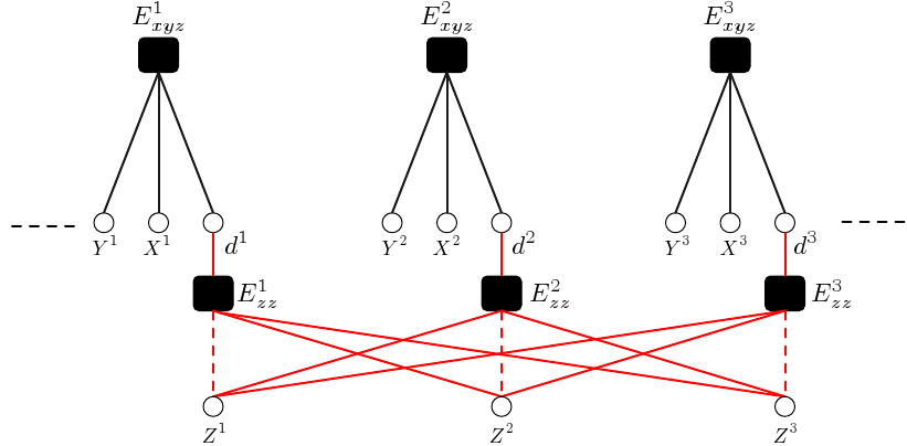
For it to be usable on new test samples without requiring excessive work, the energy function must be carefully constructed is such a way that the addition of a new sample in the arguments will not require re-training the entire system, or re-estimating some high-dimensional hidden variables. Moreover, the parameterization must be designed in such a way that its estimation on the training sample will actually result in good prediction on test samples. Training an EBRFG can be performed by minimizing the negative log conditional probability of the answer variables with respect to the parameter W. We propose an efficient training and inference algorithm for the general model. The architecture of the factor graph that was used for predicting the prices of real estate properties is shown in Figure 1 (top). The price of a house is modeled as a product of two quantities: 1. its "intrinsic" price which is dependent only on its individual features, and 2. the desirability of its location. A pair of factors Exyzi and Ezzi are associated with every house. Exyzi is non-relational and captures the sample specific dependencies. It is modeled as a parametric function with learnable parameters Wxyz. The parameters Wxyz are shared across all the instances of Exyzi. The factor Ezzi is relational and captures the dependencies between the samples via the "hidden" variables Zi. These dependencies influence the answer for a sample through the intermediary hidden variable di. The variables Zi can be interpreted as the desirability of the location of the i-th house, and di can be viewed as the estimated desirability of the house using the desirabilities of the houses related to it (those that lie in its vicinity). This factor is modeled as a non-parametric function. In particular we use a locally weighted linear regression, with weights given by a gaussian kernel. The model is trained by maximizing the likelihood of the training data, which is realized by minimizing the negative log likelihood function with respect to W and Z. However we show that this minimization reduces to
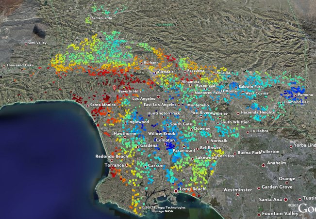
where R(Z) is a regularizer on Z (an L2 regularizer in the experiments). This is achieved by applying a type of deterministic generalized EM algorithm. It consists of iterating through two phases. Phase 1 involves keeping the parameters W fixed and minimizing the loss with respect to Z. The loss is quadratic in Z and we show that its minimization reduced to solving a large scale sparse quadratic system. We used conjugate gradient method using an adaptive threshold to minimize it. Phase 2 involves fixing the hidden variables Z and minimizing with respect to W. Since the parameters W are shared among the factors, this can be done using gradient descent. Inference on a new sample Xo involves computing its neighboring training samples, and using the learnt values of their hidden variables Z No to get an estimate of its "desirability" do; passing the house specific features Xho through the learnt parametric model to get its "intrinsic" price; and combining the two to get its predicted price. The model was trained and tested on a very challenging and diverse real world dataset that included 42,025 sale transactions of houses in Los Angeles county in the year 2004. Each house was described using a set of 18 house specific attributes like gps coordinates, living area, year build, number of bedrooms, etc. In addition, for each house, a number of neighborhood specific attributes obtained from census tract data and the school district data were also used. It included attributes like average house hold income of that area, percentage of owner occupied homes etc. The performance of the proposed model was compared with a number of standard non-relational techniques that that have been used in literature for this problem, namely nearest neighbor, locally weighted regression, linear regression, and fully connected neural network. EBRFG gives the best prediction accuracy by far, compared to other models. In addition we also plot the "desirabilities" learnt by our model (Figure 1 (bottom)). The plot shows that the model is actually able to learn the "desirabilities" of various areas in a way that is reflective of the real world situation. References
This document was translated from LATEX by HEVEA. |
|||||||||||||||||||||||||||||||||||||||||||||||||||||||||||||||