|
- Time Period: September 2003 - present.
- Participants: Fu Jie Huang, Yann LeCun (Courant Institute/CBLL), Leon Bottou (NEC Labs).
- Talks:
- Slides: End-to-End Learning of Object Categorization
with Invariance to Pose, Illumination, and Clutter.
Slides of a talk delivered at CVPR Workshop on Object Recognition,
Washington DC, June 2004.
[DjVu (2.1MB)].
- Publications:
- [LeCun, Huang, Bottou, 2004].
Learning Methods for Generic Object Recognition with Invariance to Pose and Lighting
Proceedings of CVPR 2004.
- DatasetDownload the
NORB dataset.
- Support: this project is supported by National Science
Foundation under grants numbers 0535166, and 0325463.
The recognition of generic object categories with invariance to pose,
lighting, diverse backgrounds, and the presence of clutter is one of
the major challenges of Computer Vision.
We are developing learning systems that can recognize generic object
purely from their shape, independently of pose, illumination, and
surrounding clutter.
The NORB dataset (NYU Object Recognition Benchmark) contains stereo
image pairs of 50 uniform-colored toys under 36 azimuths, 9 elevations,
and 6 lighting conditions (for a total of 194,400 individual images).
The objects were 10 instances of 5 generic categories: four-legged
animals, human figures, airplanes, trucks, and cars. Five instances
of each category were used for training, and the other 5 for testing.
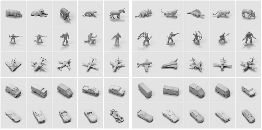 | |
The picture shows the 25 objects used for training (left panel)
and the 25 different objects used for testing (right panel).
There are five object categories: animals, human figures, airplanes,
trucks and cars.
|
Low-resolution grayscale images of the objects with various amounts of
variability and surrounding clutter were used to train and test
nearest neighbor methods, Support Vector Machines, and Convolutional
Networks, operating on raw pixels or on PCA-derived features.
|
Experiments were conducted with four datasets generated from the
normalized object images. The first two datasets were for pure
categorization experiments (a somewhat unrealistic task), while the
last two were for simultaneous detection/segmentation/recognition
experiments.
All datasets used 5 instances of each category for training and the 5
remaining instances for testing. In the normalized dataset,
972 images of each instance were used: 9elevations, 18 azimuths (0 to
340 degrees every 20 degrees), and 6 illuminations, for a total of
24,300 training samples and 24,300 test samples. In the various
jittered datasets, each of the 972 images of each instance were
used to generate additional examples by randomly perturbing the
position ([-3, +3] pixels), scale (ratio in [0.8, 1.1]), image-plane
angle ([-5, 5] degrees), brightness ([-20, 20] shifts of gray levels),
contrast ([0.8, 1.3] gain) of the objects during the compositing
process. Ten drawings of these random parameters were drawn to
generate training sets, and one or two drawings to generate test sets.
|
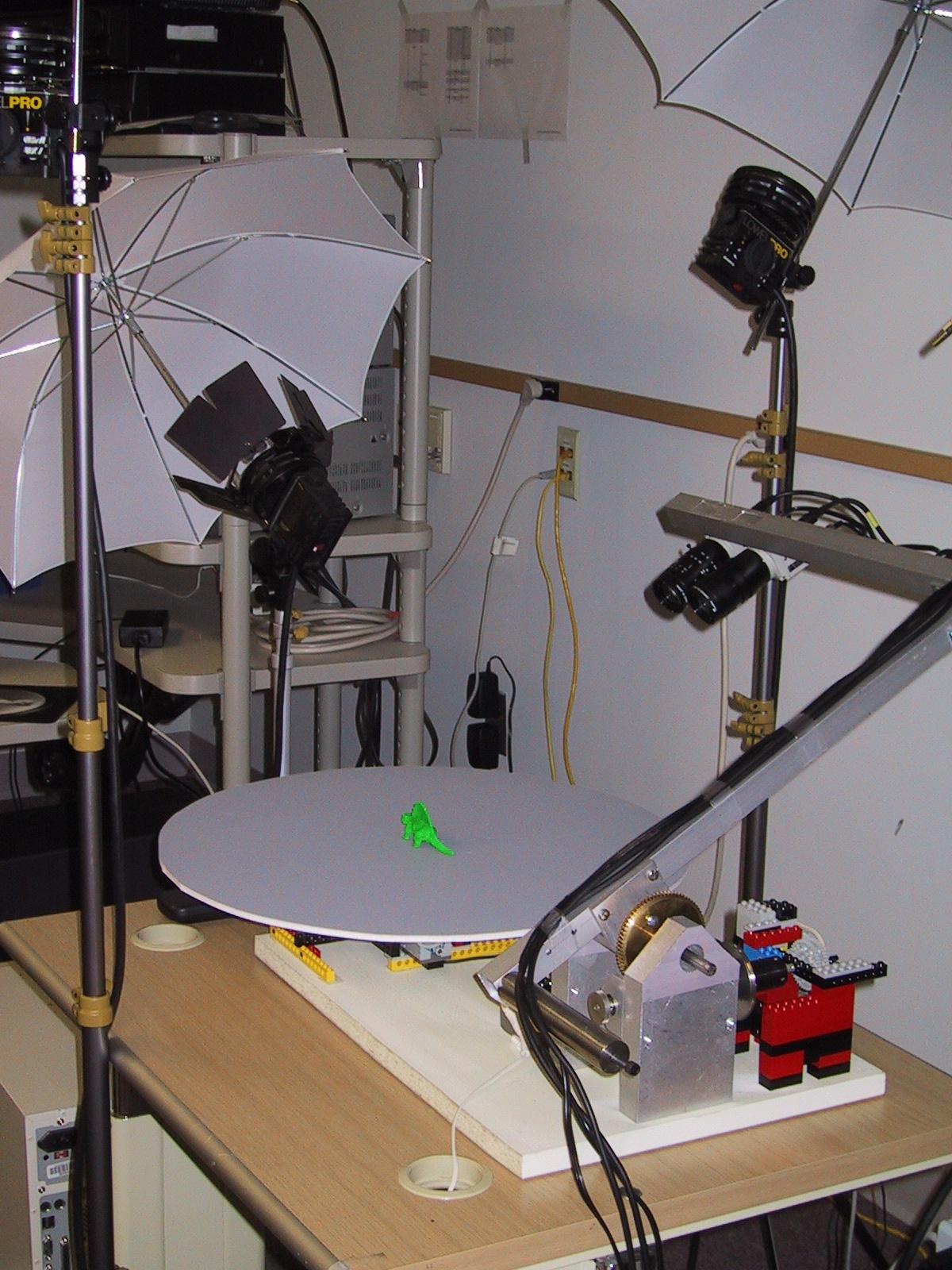
| [click picture to enlarge] |  | |
Image capturing setup. | |
|
In the textured and cluttered datasets, the objects were
placed on randomly picked background images. In those experiments, a
6-th category was added: background images with no objects (results
are reported for this 6-way classification). In the textured
set, the backgrounds were placed at a fixed disparity, akin to a back
wall orthogonal to the camera axis at a fixed distance. In the cluttered datasets, the disparities were adjusted and randomly
picked so that the objects appeared placed on highly textured
horizontal surfaces at small random distance from that surface. In
addition, a randomly picked ``distractor'' object from the training
set was placed at the periphery of the image.
|
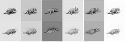 | |
Examples of the various lighting conditions for two elevations) |
|
- normalized-uniform set: 5 classes, centered, unperturbed objects on uniform
backgrounds. 24,300 training samples, 24,300 testing samples.
- jittered-uniform set: 5 classes, random perturbations, uniform backgrounds.
243,000 training samples (10 drawings) and 24,300 test samples (1 drawing)
- jittered-textured set: 6 classes (including one background class)
random perturbation, natural background textures at fixed disparity.
291,600 training samples (10 drawings), 58,320 testing samples (2 drawings).
- jittered-cluttered set: 6 classes (including one background class),
random perturbation, highly cluttered background images at random disparities,
and randomly placed distractor objects around the periphery.
291,600 training samples (10 drawings), 58,320 testing samples (2 drawings).
|
| [click picture to enlarge] | 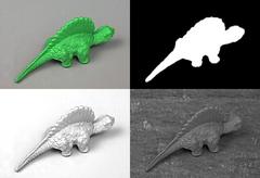 | |
Compositing process. top left: raw image; top right: chroma-keyed
object mask; bottom left: cast shadow coefficient mask; bottom right:
composite image with cast shadow. | |
Occlusions of the central object by the distractor occur occasionally
in the jittered cluttered set. Most experiments were performed in
binocular mode (using left and right images), but some were performed
in monocular mode. In monocular experiments, the training set and test
set were composed of all left and right images used in the
corresponding binocular experiment. Therefore, while the number of
training samples was twice higher, the total amount of training data
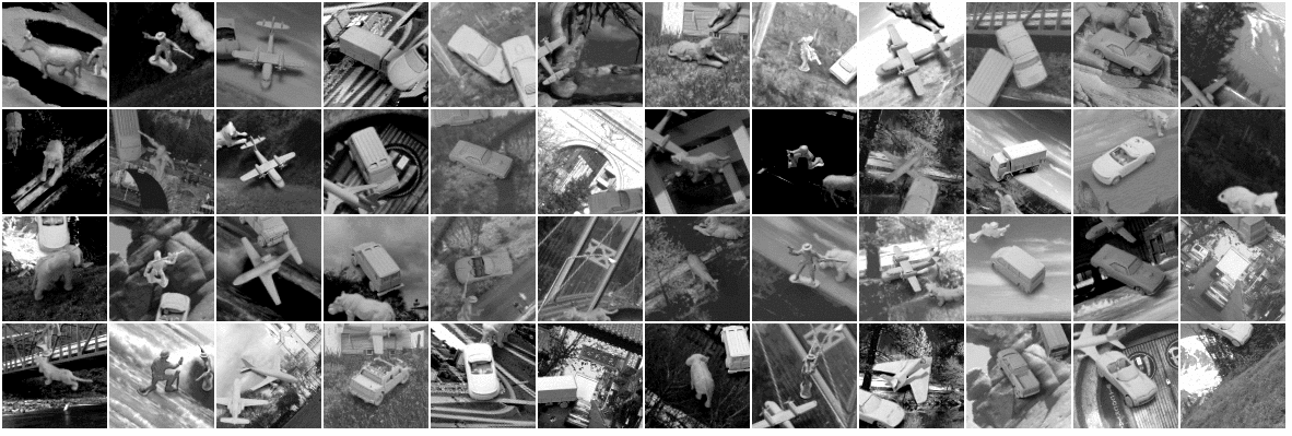
was identical. Examples from the jittered-textured and
jittered-cluttered training set are shown below
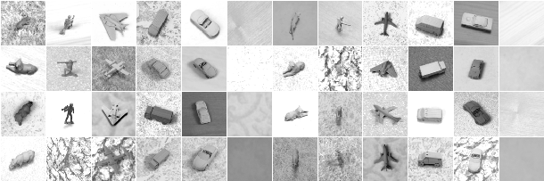 | | Examples from the jittered-textured |
On the Normalized-Uniform Dataset
| Classifier | Error Rate |
| Linear Classifier, binocular | 30.2% error |
| K-Nearest Neighbors on raw stereo images | 18.4% error |
| K-Nearest Neighbors on 95 PCA features | 16.6 error |
| Pairwise Support Vector Machine on raw stereo images | NO CONVERGENCE |
| Pairwise SVM on 48x48 monocular images | 13.9% error |
| Pairwise SVM on 32x32 monocular images | 12.6% error |
| Pairwise SVM on 95 PCA features | 13.3 error |
| Convolutional Network "LeNet7" | 6.6% error |
| Convolutional Network "LeNet7" with pose manifold | 6.2% error |
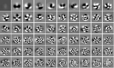 | |
The first 60 principal components extracted from the
normalized-uniform training set. Unlike with eigen-faces these
"eigen-toys" are not recognizable and have symmetries because the
objects are seen from every angle in the training set. |
On the Jittered-Cluttered Dataset
| Classifier | Error Rate |
| Convolutional Network "LeNet7", binocular | 7.8% error |
| Convolutional Network "LeNet7", monocular | 20.8% error |
| [click picture to enlarge] |
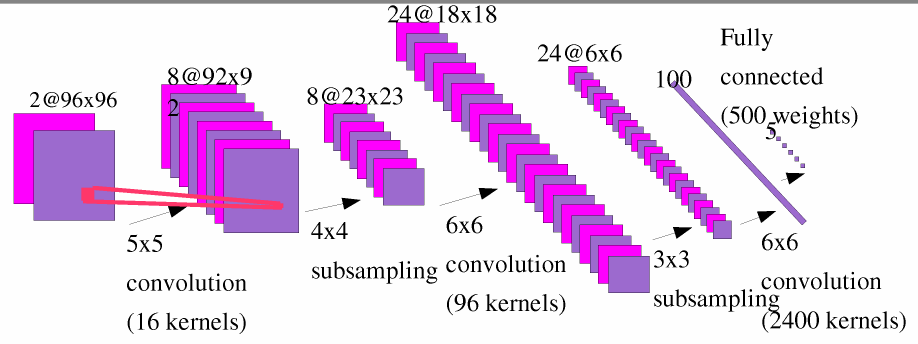 |
| Architecture of the convolutional net "LeNet 7". This network has
90,857 trainable parameters and 4.66 Million connections.
Each output unit is influenced by a receptive field of 96x96 pixels
on the input.
|
 | |
Learned kernels from the first layer of the binocular convolutional
network. |
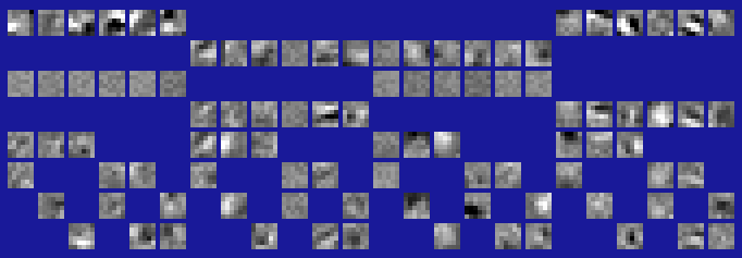 | |
Learned kernels from the third layer of the binocular convolutional
network. |
The convolutional network can be very efficiently applied to all
locations on a large input image. For example, applying LeNet 7 to a
single 96x96 window requires 4.66 Million multiply-accumulate
operations. But applying LeNet 7 to every 96x96 windows, shifted every
12 pixels, over a 240x240 image (169 windows) requires only 47.5
Million multiply-accumulate operations. Applying a non-convolutional
classifier with the same complexity to every such 96x96 window would
consume 788 Million operations (4.66 million times 169).
The network can be applied to images at multiple scales to
ensure scale invariance.
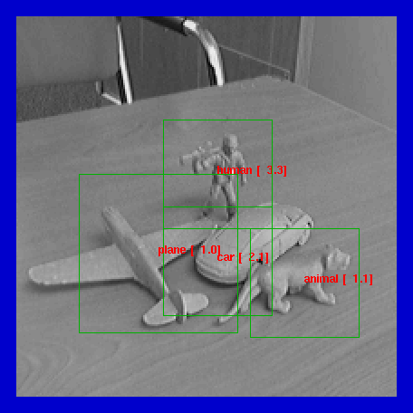
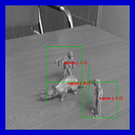
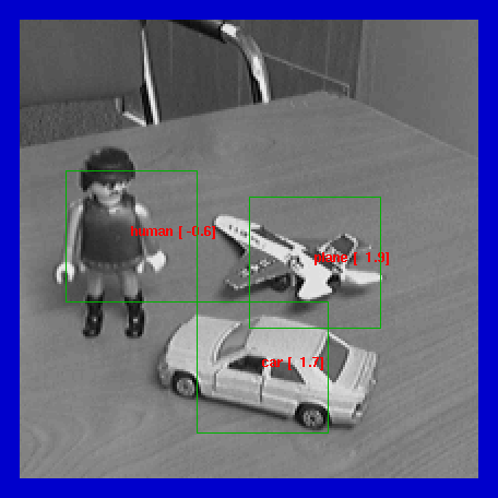
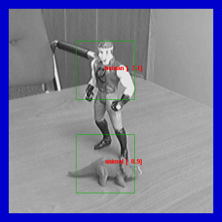
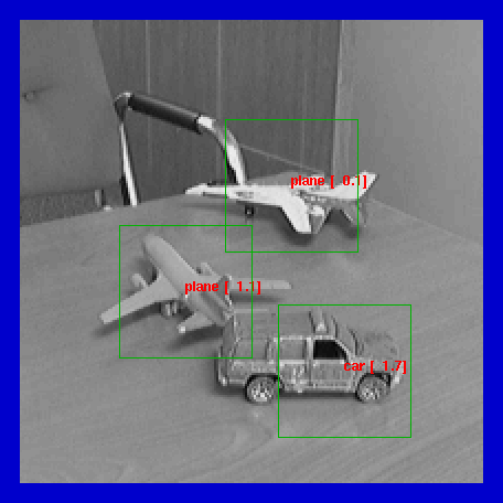
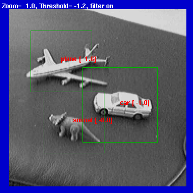
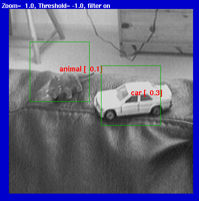
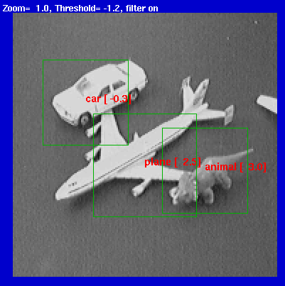
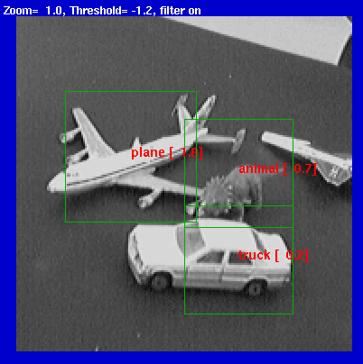
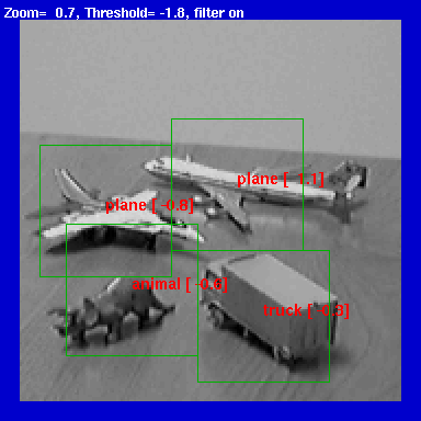
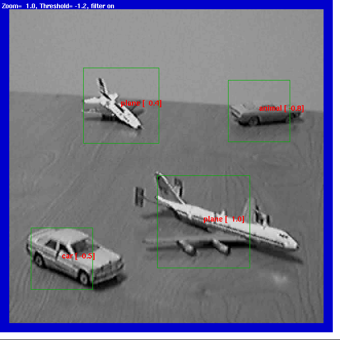
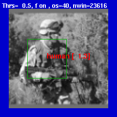
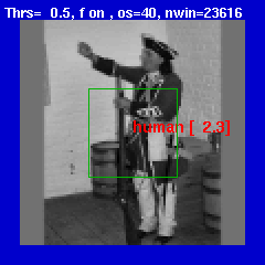
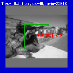
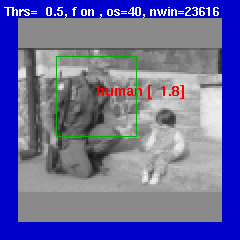
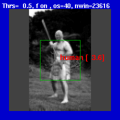
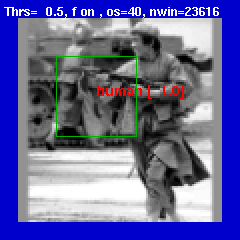
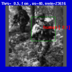
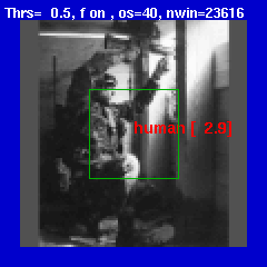
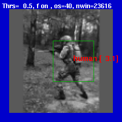
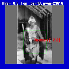
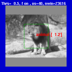
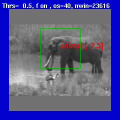
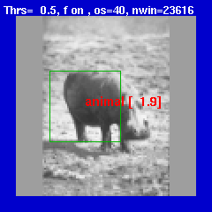
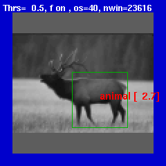
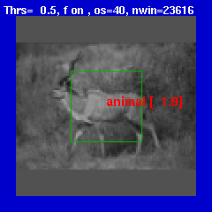
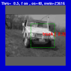
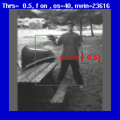
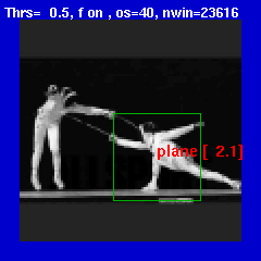
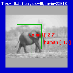
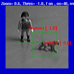
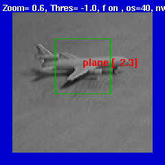
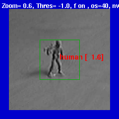
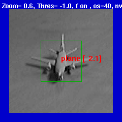
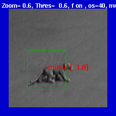
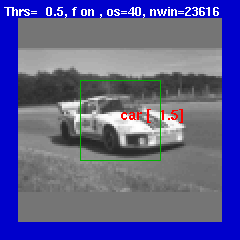
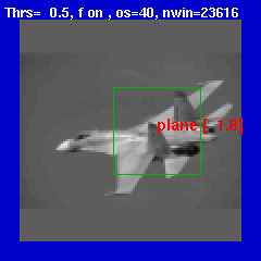
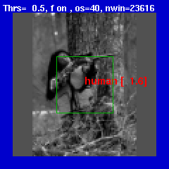
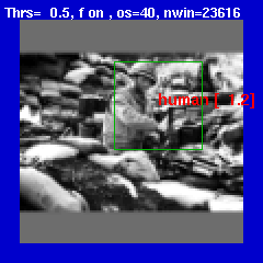
A system was built around LeNet 7, that can detect and recognize
objects in natural images. The system runs in real time (a few
frames per second) on a laptop connected to a USB camera. Examples of
outputs from that system are shown below.
Scenes with objects from the NORB dataset
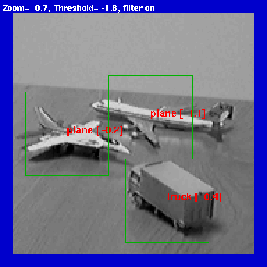
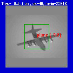
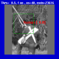
Various scenes with other objects
Natural Scenes
NOTE: The system was not trained on natural images.
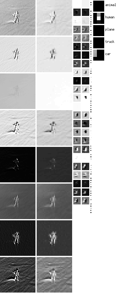
A few mistakes
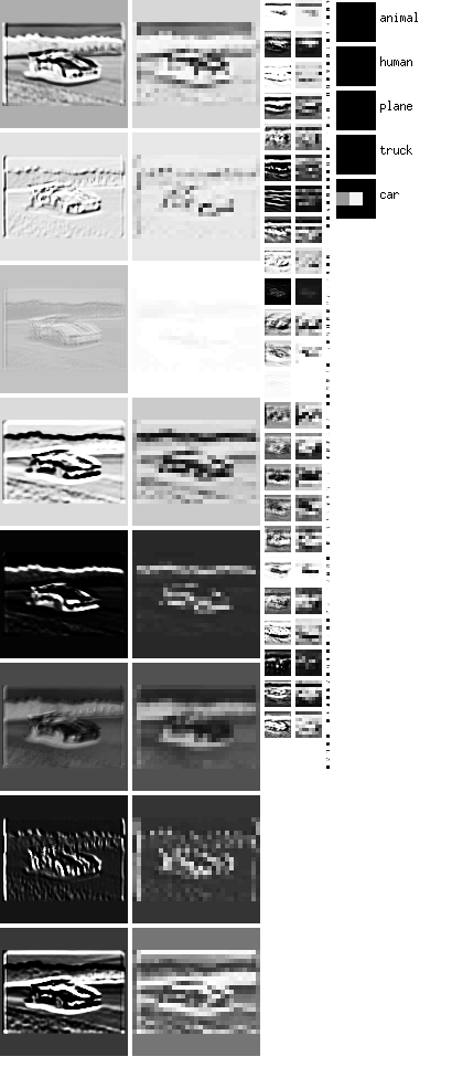
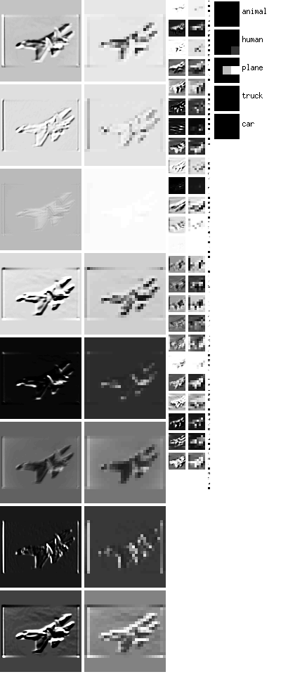
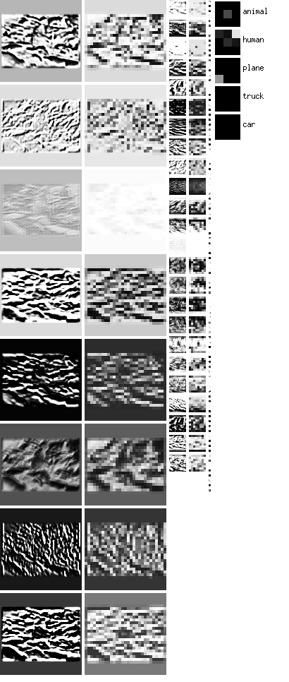
Examples with the Internal State of the Convolutional Network
|
|