|
- Time Period: September 2003 - present.
- Participants: Yann LeCun, Sumit Chopra, Raia Hadsell, Fu-Jie
Huang, Marc'Aurelio Ranzato (Courant Institute/CBLL)
| Tutorials, Talks, and Videos |
- [LeCun et al
2006]. A Tutorial on Energy-Based Learning, in
Bakir et al. (eds) "Predicting Structured Outputs", MIT Press
2006: a 60-page tutorial on energy-based learning, with an
emphasis on structured-output models. The tutorial includes
an annotated bibliography of discriminative learning, with
a simple view of CRF, maximum-margin Markov nets, and
graph transformer networks.
- [LeCun and Huang, 2005].
Loss Functions for Discriminative Training of Energy-Based Models.
Proc. AI Stats 2005.
- [Osadchy, Miller, and
LeCun, 2004] Synergistic Face Detection and Pose Estimation
Proc. NIPS 2004. This paper uses an energy-based model methodology
and contrastive loss function to detect faces and simultaneously
estimate their pose.
Probabilistic graphical models associate a probability to each
configuration of the relevant variables. Energy-based
models (EBM) associate an energy to those configurations,
eliminating the need for proper normalization of probability
distributions. Making a decision (an inference) with an EBM consists
in comparing the energies associated with various configurations of
the variable to be predicted, and choosing the one with the smallest
energy. Such systems must be trained discriminatively to associate
low energies to the desired configurations and higher energies to
undesired configurations. A wide variety of loss function can be used
for this purpose. We give sufficient conditions that a loss function
should satisfy so that its minimization will cause the system to
approach to desired behavior.
An EBM can be seen as a scalar energy function of three
(vector) variables E(Y,Z,X), parameterized by a set of trainable
parameters W. X is the input, which is always observed (e.g. pixels
from a camera), Y is the set of variables to be predicted (e.g. the
label of the object in the input image), and Z is a set of latent
variables that are never directly observed (e.g. the pose of the
object).
Performing an inference consists in observing an X, and looking
for the values of Z and Y that minimize the energy E(Y,Z,X).
Given a training set S={ (X1,Y1), (X2,Y2),....(Xp,Yp) },
training an EBM consists in "digging holes" in the energy surface
at the training samples (Xi,Yi), and "building hills" everywhere else.
This process will make the desired Yi become a minimum of the
energy for the given Xi.
The main question is how to design a loss function so that
minimizing this loss function with respect to the parameter
vector W will have the effect of digging holes and building
hills at the required places in the energy surface.
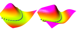
In the following, we demonstrate how various types
of loss functions shape the energy surface.
The task to learn is the square function Y=X^2.
In the animations, the blue spheres indicate the
location of training samples (a subset of the training
samples). A good loss function will shape the energy
surface so that the blue spheres are minima (over Y)
of the energy for a given X.
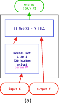
Here, we demonstrate how "traditional" supervised learning
applied to a traditional neural net (viewed as an EBM)
shapes the energy surface. The EBM architecture is a traditional
2-layer neural net with 20 hidden units, followed by a cost
module that measures the L1 distance between the network output
and the desired output Y. The value of Y that minimizes the energy
is simply equal to the neural net output.
The loss function used here is simply the average squared energy
over the training set. This is the traditional square loss
used in conventional neural nets. With this architecture, the shape of
the energy as a function of Y is constant (it's a V-shaped
function), only the location of its minimum can change.
Therefore, digging a hole at the right Y will automatically
make the other values of Y have higher energies.
|
 |
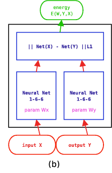
In this second example, we use a different architecture,
shown at right, where both X and Y are fed to neural nets.
The outputs of the nets are fed to an L1 distance module.
The loss function used here is again the average squared energy
over the training set. The shape of the energy as a function of Y
is no longer constant, but depends on the neural net on the right.
A catastrophic collapse happens: the two neural nets
are perfectly happy to simply ignore X and Y and produce
identical, constant outputs (the flat green surface is the
solution, the orange-ish surface is the random initial condition).
The loss function pulls down on the blue spheres, but nothing
is pulled up, and nothing prevents the energy surface from becoming
flat. It does become flat. Hence the collapse.
|
 |
In this third example, we use the same dual net architecture,
but we use the so-called square-square generalized margin loss
function which not only pulls down on the blue spheres, but also
pulls up on points on the surface some distance away from the blue
spheres.
The point being pulled up for a given X is the Y with the
lowest energy that is at least 0.3 away from the desired Y.
This time, no collapse occurs, and the energy surface
takes the right shape.
|
|
In this fourth example, we use the same dual net architecture,
trained with the negative-log-likelihood loss function.
This loss pulls down on the blue spheres, and pulls up on
all points of the surface, pulling harder on points with lower
energy.
This is the loss used to train traditional probabilistic models
by maximizing the conditional likelihood of all the Yi given
all the Xi.
Again, no collapse occurs, but the computation is considerably
more expensive than in the previous example, because we need to
compute the integral over all values of Y of the derivative of
the energy with respect to W (the derivative of the log partition
function).
Also, this loss function makes the energies of undesired Y grow
without bounds, and it does not pull the energies of the blue
spheres toward zero (only relative values matter).
|
|
|
|