Improvements on pLSA and their application to Google data
Probabilistic Latent Semantic Analysis (pLSA)
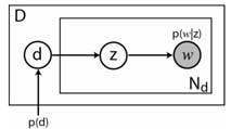
pLSA is a bag of words type model, proposed by Hoffman [1]. It was applied to visual data by Sivic et al. [2] and Fei-Fei et al. [3] (the latter using a related method, LDA). For more details on it, please see the slides and code from our ICCV 2005 short course. For our purposes, documents will correspond to images, topics to objects within the image and words to vector quantized appearance of regions found by a region detector. For reference, the graphical model of pLSA is shown below.
Incorporating Spatial Information
The obvious problem with applying pLSA directly to visual data is that the spatial information of each visual word is not used. We propose two simple increments to the model to incorporate spatial information.
ABS-pLSA
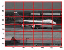
The simplest way to bring in location information is to impose a discrete location grid on the image and then have a joint density on location and visual words. In other words, each spatial bin has its own distribution over appearance. The graphical model for this approach (which we name ABS-pLSA) is given below, along with a visualization of the 6x6 grid we use in our experiments.
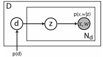
The obvious drawback to this model is that it is not able to handle a translation or scaling of the object within the image. However, we will use this model as a baseline for TSI-pLSA, our next model.
TSI-pLSA
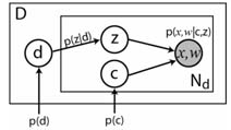
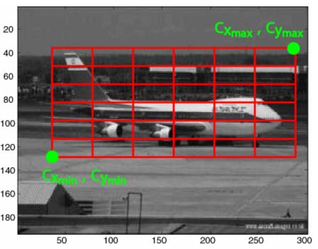
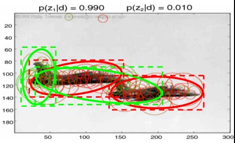
TSI-pLSA introduces a latent variable c which describes a bounding box within the image. Within that box we have a discrete location distribution as before. The rest of the image is considered to be one large spatial bin. To avoid an exhaustive search over all possible bounding boxes, we use an appearance-only model (plain pLSA) to propose a set of bounding boxes. This is done by fitting a series of mixture of Gaussian models to the regions within the image, using the variance of the Gaussian to determine the extent of the bounding box. The figure on the left below shows the graphical model for TSI-pLSA. The figure in the center shows a schematic of the floating bounding box within the image. The figure on the right shows the bounding boxes proposed by a mixture of Gaussians models fit to the visual words of an appearance-only model.
Comparing the Different Models on the PASCAL Datasets
We have outlined three different models, pLSA, ABS-pLSA and TSI-pLSA. Before applying them to Google data, we first evaluate them on manually gathered training data in the form of the PASCAL 2005 datasets. Below is a table showing the classification performance of the three versions on two of the classes. These datasets have a wide range of pose variation, hence the global location model of ABS-pLSA is unlikely to offer much improvement over pLSA.The figure quoted in the table is the equal error rate, hence a lower number is better. The ABS-pLSA performs comparably to the pLSA model, but the TSI-pLSA shows a marked improvement.
| Equal error rate (%) | pLSA | ABS-pLSA | TSI-pLSA |
| PASCAL Cars | 31.7 | 30.8 | 25.8 |
| PASCAL Motorbikes | 33.7 | 30.2 | 25.7 |
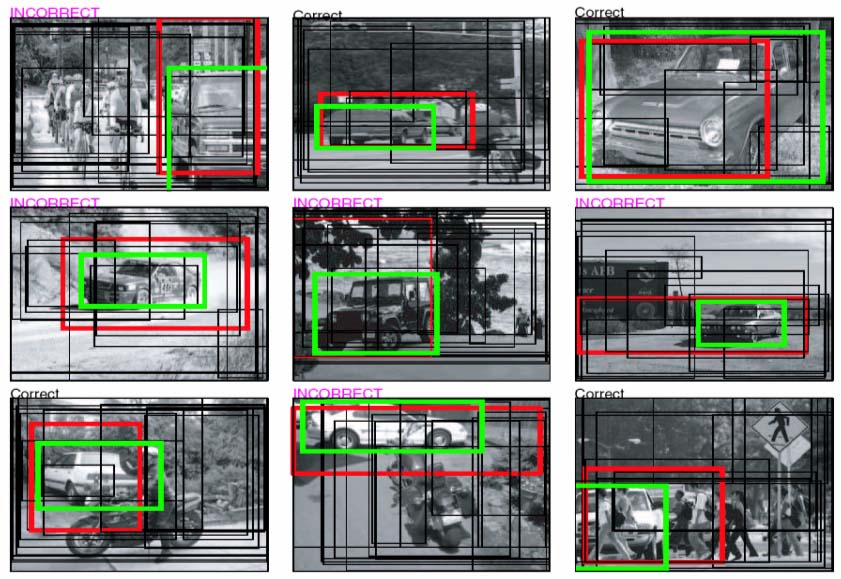
We also evaluated TSI-pLSA in a localization task. Below we show some sample images. The green box is the ground truth location of the object; the red box is the location as predicted by TSI-pLSA. The black rectangles show the proposed bounding boxes.
Applying the Models to Google Data
To apply the models to Google, we require two important extra pieces of information:
- The correct number of topics to use
- How to select the topic that has learnt the visual category corresponding to the query term
For the first point, we determine via experimentation that 8 topics work well, roughly reflecting that the portion of good images is in the region of 1/8th of the data. The second point is trickier - we would normally need a validation set to make such a decision. Since we do not have any labeled data we automatically build a noisy validation set, using this method. Having trained a model on Google data, we apply each of the 8 topics to the validation set and pick the best performing one.
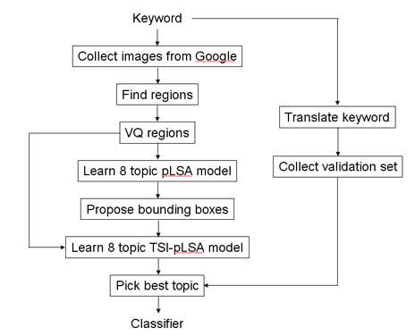
The whole training procedure for TSI-pLSA is summarized in the flowchart below:
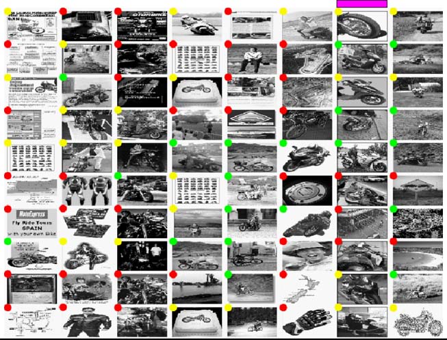
Below we show the results of training a pLSA model on data collected from Google using the query "motorbike". Each column shows the top 10 images for each topic. The colored dot in the top-left corner of each image shows the ground-truth label of each image (used only for evaluation purposes). The magenta bar indicates the topic selected by the noisy validation set. While there is some clustering of the data, none of the topics closely relate to motorbikes.
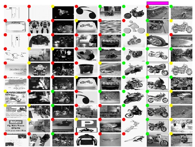
Below we show results of training a TSI-pLSA model on the same data. Note that the topics now seem more coherent. The automatically selected topic seems to contain a lot of motorbike images. The topic to its left also contains motorbikes but from a different viewpoint.
Example Models
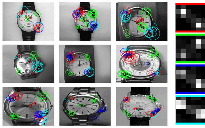
It is informative to look at the models obtained by training on Google data. Of the seven classes we evaluated, wrist watch had the largest portion of good images. The TSI-pLSA model for wrirst watch is shown below. The images on the left are hand-gathered test images (deliberately picked to have little clutter, so as to see clearly what the model is selecting from the object). Superimposed on them are a subset of the regions belonging to the top 4 visual words as associated with the automatically selected topic. On the right the spatial location distribution within the floating sub-window is shown for each of the top 4 words, their border colors corresponding to the regions show on the left. Taking the visual word highlighted in red, the spatial distribution is distinctly bi-modal. Examining the images, it seems that this word is picking out the oriented edge of the bezel. The green words seem to also pick out the bezel, but from the opposite orientation.
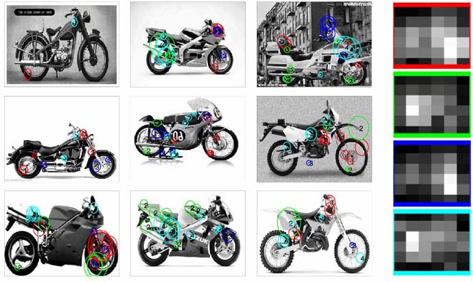
Below we show the TSI-pLSA model for motorbikes. The model here is less distinct, with the spatial distributions more diffused, but still far from uniform. It is important to realize that the model is using a 1000 or so regions per image rather than the handful we show here.
We now compare the three pLSA variants with a Constellation Model in a variety of experiments on the main page.
References
[1] Probabilistic Latent Semantic Indexing. T. Hofmann. In SIGIR '99: Proceedings of the 22nd Annual International ACM SIGIR Conference on Research and Development in Information Retrieval, August 15-19, 1999, Berkeley, CA, USA, pages 50-57. ACM, 1999.
[2] Discovering Object Categories in
Image Collections. J. Sivic, B. Russell, A. Efros, A. Zisserman, and W.
Freeman. Technical Report A. I. Memo 2005-005, Massachusetts Institute of
Technology, 2005.
[3] A Bayesian Hierarchical Model for
Learning Natural Scene Categories. L. Fei-Fei and P. Perona. Proceedings
of the IEEE Conference on Computer Vision and Pattern Recognition,
San Diego, CA, volume 2, pages 524-531, June 2005.