Homework 6, assigned Nov 10, due Nov 23

This homework is due the day before Thanksgiving, although we do not have class Nov 23. You can leave it under my office door any time. If it is difficult for you to bring the homework to NYU, let me know by email and we'll make some other arrangement.

Interpolation

1. Take a look at this plot. There are are 21 (x,y) pairs plotted approximately in the shape of an S. The data values, which I obtained by entering the points in a Matlab graphics window using ginput, are here; save this file as S.mat and then load the data into Matlab with load S. The purpose of this assignment is to plot a smooth curve through these points in the x-y plane. However, we can't write y as a function of x or x as a function of y. Instead, we can determine a pair of smooth functions, one to interpolate the x-coordinates as a function of t, and one to interpolate the y-coordinates as a function of t, where you can think of t as "time", as the curve is drawn from start to finish in the x-y plane, running, in this case, from t=1 to t=21.

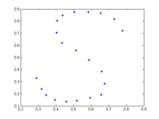
   Write a function that takes as input a set of points such as the S points, and plots 3 different interpolating curves in 3 different graphics windows: (1) using polynomial interpolation, (2) using piecewise cubic Hermite interpolation, and (3) using cubic splines. You can use any method you want to compute these. For (1) I suggest either setting up a Vandermond matrix and solving it, or using polyinterp, which uses the Lagrange formulation. For (2), use pchip or pchiptx. For (3), use spline or splinetx. Recall that the polyinterp, pchiptx and splinetx routines, along other related files and the accompanying text book, are available at Moler's website. All these routines have similar interfaces: the first argument specifies the independent variable at the interpolation points, which here is called t (the integers 1 through 21 in the case of the S points), the second provides the dependent variable values, which here are either x or y, at the interpolation points, and the third provides additional independent variable values at which the interpolating function is supposed to be evaluated, for example, 1: 0.1: 21 or equivalently linspace(1,21,201). Your plots should be plots in the x-y plane, not of x as a function of t or y as a function of t. Plot the interpolation points with the symbol '*' and the interpolating (in-between) points, with '.' or '-', but be aware that if you use '-', the plotter does additional linear interpolation between the points. The function should be written to handle any set of points. In addition to the results for the S points, print results for another set of points that you make up yourself (try to think of something with an interesting smooth shape).

2. The cubic spline routines solve a tridiagonal system to obtain the derivative values at the knots, as we discussed in class. The splinetx routine does this by calling tridisolve, which we studied in detail. This routine does not use pivoting because the linear system set up by splinetx is known to be diagonally dominant.

   Modify tridisolve (available here) so that it is suitable for solving any tridiagonal system, by introducing partial pivoting (row interchanges). As discussed in class, that means one more array is needed to store the second superdiagonal of the matrix, to store the fill-in (nonzeros that are introduced by the elimination). Be sure you include comments in the program, which may as well document the original code as well as the new lines. Test the program on some tridiagonal systems with some zeros or small numbers on the diagonal. How much CPU time is needed to solve a tridiagonal system with size one million? Does the row pivoting increase the running time substantially? Compare the accuracy and speed with using Matlab's sparse matrix system i.e. x = T\d where T = spdiags([[a; 0] b [0; c]],[-1 0 1],n,n), as suggested in the comments of tridisolve. Here the [-1 0 1] refers to the first subdiagonal, diagonal, and superdiagonal of T; with this approach, the fill-in is taken care of automatically so you don't have to allocate space for the second superdiagonal.